List of project topics
Please find a tentative list here. Some more links might be added in the next few days. Feel free to pick a topic outside this list. Remember, the deadline for *choosing* a project (and letting me know, along with partner information) is Monday, 27th March.
Homework problems
We will have a stream of homework problems, following every class. Since this is an advanced graduate level class, solving these problems right after class will (hopefully) help you understand the material better.
Part I: Foundations of Learning Theory
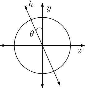
Problem 1. Consider the problem of classifying points in the two-dimensional plane, i.e., $\mathcal{X} = \mathbb{R}^2$. Suppose that the (unknown) true label of a point $(x, y)$ is given by sign$(x)$ (we define sign$(0) = +1$, for convenience). Suppose the input distribution $\mathcal{D}$ is the uniform distribution over the unit circle centered at the origin.
(a) Consider the hypothesis $h$ as shown in the figure below ($h$ classifies all the points on the right of the line as $+1$ and all the points to the left as $-1$). Compute the risk $L_{\mathcal{D}}(h)$, as a function of $\theta$ (which is, as is standard, given in radians).
(b) Suppose we obtain $1/\theta$ (which is given to be an integer $\ge 2$) training samples (i.e., samples from $\mathcal{D}$, along with their true labels). What is the probability that we find a point whose label is "inconsistent" with $h$? Can you bound this probability by a constant independent of $\theta$?
(c) Give an example of a distribution $\mathcal{D}$ under which $h$ has risk zero.
Problem 2. Suppose $A_1, A_2, \dots, A_n$ are events in a probability space.
(a) Suppose $\Pr[A_i] = \frac{1}{2n}$ for all $i$. Then, show that the probability that none of the $A_i$'s occur is at least $1/2$.
(b) Give a concrete example of events $A_i$ for which $\Pr[A_i] = \frac{1}{n-1}$ for all $i$, and the probability that none of them occur is zero.
(c) Suppose $n \ge 3$, and $\Pr[A_i] = \frac{1}{n-1}$, but the events are all independent. Show that the probability that none of them occur is $\ge 1/8$.
Problem 3. In our proof of the no-free lunch theorem, we assumed the algorithm $A$ to be deterministic. Let us now see how to allow randomized alorithms. Let $A$ be a randomized map from set $X$ to set $Y$. Formally, this means that for every $x \in X$, $A(x)$ is a random variable, that takes values in $Y$. Suppose $|X| < c |Y|$, for some constant $c<1$.
(a) Show that there exists a $y \in Y$ such that $\max_{x \in X} \Pr[ A(x) = y] \le c$.
(b) Show that this implies that for any distribution $\mathcal{D}$ over $X$, $\Pr_{x \sim \mathcal{D}} [A(x) = y] \le c$ (for the $y$ shown to exist in part (a)).
Problem 4. Recall that the VC dimension of a hypothesis class $\mathcal{H}$ is the size of the largest set that it can "shatter".
(a) Consider the task of classifying points on a 2D plane, and let $\mathcal{H}$ be the class of axis parallel rectangles (points inside the rectangle are "+" and points outside are "-"). Prove that the VC dimension of $\mathcal{H}$ is 4.
(b) This time, let $\mathcal{X} = \mathbb{R}^d \setminus \{0\}$ (origin excluded), and let $\mathcal{H}$ be the set of all hyperplanes through the origin (points on one side are "+" and the other side are "-"). Prove that the VC dimension of $\mathcal{H}$ is $\le d$.
(HINT: consider any set of $d+1$ points. They need to be linearly dependent. Now, could it happen that $u, v$ are "+", but $\alpha u + \beta v$ is "-" for $\alpha, \beta \ge 0$? Can you generalize this?)
(c) (BONUS) Let $\mathcal{X}$ be the points on the real line, and let $\mathcal{H}$ be the class of hypotheses of the form $\text{sign}(p(x))$, where $p(x)$ is a polynomial of degree at most $d$ (for convenience, define sign$(0) = +1$). Prove that the VC dimension of this class is $d+1$. (HINT: the tricky part is the upper bound. Here, suppose $d=2$, and suppose we consider any four points $x_1 < x_2 < x_3 < x_4$. Can the sign pattern $+,-,+,-$ arise from a degree $2$ polynomial?)
Problem 5. In the examples above (and in general), a good rule of thumb for the VC dimension of a function class is the number of parameters involved in defining a function in that class. However, this is not universally true, as illustrated in this problem: let $\mathcal{X}$ be the points on the real line, and define $\mathcal{H}$ to be the class of functions of the form $h_\theta := \text{sign}( \sin \theta x)$, for $\theta \in \mathbb{R}$. Note that each hypothesis is defined by the single parameter $\theta$.
Prove that the VC dimension of $\mathcal{H}$ is infinity.
So where does the "complexity" of the function class come from? (BONUS) prove that if we restrict $\theta$ to be a rational number whose numerator and denominator have at most $n$ bits, then the VC dimension is $O(n)$.
***** This concludes the problems for HW1. The five problems above are due on Wednesday Feb 15 (in class). *****
Problem 6. (Convexity basics) For this problem, let $f$ be a convex function defined over a convex set $K$, and suppose the diameter of $K$ is $1$.
(a) Let $x \in K$, and suppose $f(x) = 2$ and $\lVert \nabla f(x)\rVert = 1$. Give a lower bound on $\min_{z \in K} f(z)$.
(b) Let $x^*$ be the minimizer of $f$ over $K$ (suppose it is unique), and let $x$ be any other point. The intuition behind gradient descent is that the vector: $- \nabla f(x)$ points towards $x^*$. Prove that this is indeed true, in the sense that $\langle \nabla f(x), x - x^* \rangle \ge 0$ (i.e., the negative gradient makes an acute angle with the line to the optimum).
(c) Suppose now that the function $f$ is strictly convex, i.e.,
$f(\lambda x + (1-\lambda) y) < \lambda f(x) + (1-\lambda) f(y)$ (strictly), for all $x \ne y$, and $0<\lambda < 1$.
Prove that all the maximizers of $f$ over $K$ lie on the boundary of $K$. [Hint: You may want to use the definition that a point $x$ is not on the boundary iff there exist points $y, z \in K$ such that $x = (y+z)/2$.]
Problem 7. (Gradient descent basics)
(a) Give an example of a function defined over $\mathbb{R}$, for which for any step-size $\eta > 0$ (no matter how small), gradient descent with step size $\eta$ oscillates around the optimum point (i.e., never gets to distance $< \eta/4$ to it), for some starting point $x \in \mathbb{R}$.
(b) Consider the function $f(x, y) = x^2 + \frac{y^2}{4}$, and suppose we run gradient descent with starting point $(1,1)$, and $\eta = 1/4$. Do we get arbitrarily close to the minimum? Experimentally, find the threshold for $\eta$, beyond which gradient descent starts to oscillate.
(c) Why is the behavior similar to that in part (a) (oscillation for every $\eta$) not happening in part (b)?
Problem 8. (Stochastic gradient descent) Suppose we have points $(a_1, b_1), (a_2, b_2), \dots, (a_n, b_n)$ in the plane, and suppose that $|a_i| \le 1$, and $|b_i| \le 1$ for all $i$. Let $f(x, y) = \frac{1}{n} \sum_{i=1}^n f_i(x, y)$, where $f_i(x, y) = (x - a_i)^2 + (y - b_i)^2$.
(a) What is the point $(x, y)$ that minimizes $f(x, y)$?
(b) Suppose we perform gradient descent (on $f$) with step size $0 < \eta< 1$. Give a geometric interpretation for one iteration.
(c) Now suppose we perform stochastic gradient descent with fixed step size $0 < \eta <1$, and by picking $i$ at random in $\{1, \dots, n\}$, and moving along the gradient of $f_i$ (as in SGD seen in class). After $T$ steps, for $T$ large enough, can we say that we get arbitrarily close to the optimum? (Provide a clear explanation.) [Hint: Remember $\eta$ is fixed.]
(d) Pick $n=100$ random points in $[-1,1]^2$ (uniformly), and run SGD for fixed $\eta = 1/2$, as above. Write down what the distance to optimum is, after T = 10, T=100, and T=1000 iterations (if you want to be careful, you should average over 5 random choices for the initialization.) Now consider a dropping step size $\eta_t = 1/t$, and write down the result for $T$ as above.
Problem 9. (Numeric accuracy in MW updates) Consider the randomized experts setting we saw in class (we maintain a distribution over experts at each time, and the loss of the algorithm at that time is the expected loss over the distribution). Consider a setting where the experts predict $0/1$, and the loss is either $0$ or $1$ for each expert. We saw how to update the probabilities (multiply by $e^{-\eta}$ if an expert makes a mistake, keep unchanged otherwise, and renormalize).
One of the common issues here is that numeric errors in such computations tend to compound if not done carefully. Suppose we have $N$ experts, and we start with a uniform distribution over them. Let $p_t^{(i)}$ denote the probability of expert $i$ at time $t$, for the ``true'' (infinite precision) multiplicative weight algorithm, and let $q_t^{(i)}$ denote the probabilities that the `real life' algorithm uses (due to precision limitations).
(a) One simple way to deal with limited precision is to zero out weights that are ``too small''. Specifically, suppose we set $q_t^{(i)} = 0$ if $ q_t^{(i)}/ \max_j q_t^{(j)} < \epsilon $, for some precision parameter $\epsilon$ (such changes frequently occur due to roundoff). Other than this, suppose that the $q_t^{(i)}$ are updated accurately. Prove that in this case, we cannot hope to achieve any non-trivial regret bound. Specifically, for large enough $T$, the algorithm could have error $T(1-o(1))$, while the best expert may have error $o(T)$. [Hint: in this case, we are ``losing'' all information about an expert.]
(b) A simple way to overcome this is to avoid storing probabilities, but instead to maintain the number of mistakes $m_t^{(i)}$. Prove how this suffices to recover the probabilities $p_t^{(i)}$ (assuming infinite precision arithmetic).
(c) It turns out that we can use the idea in part (b) to come up with a distribution $q_t$ such that (1) $q_t$ differs from $p_t$ by $ < \epsilon$ in the $\ell_1$ norm, i.e., $\sum_{i} |p_t^{(i)} - q_t^{(i)}| < \epsilon$, and (2) $q_t$ can be represented using finite precision arithmetic (the precision depends on $\epsilon$).
Now, suppose we use $q_t$ to sample (as a proxy for $p_t$), show that the expected number of mistakes of the resulting algorithm is bounded by $(1+\eta) \min_i m_T^{(i)} + O(\log N/\eta) + \epsilon T$.
(d) The bound above is not great if there is an expert who makes very small number of mistakes, say a constant (because we think of $\epsilon$ as a constant, and $T$ as tending to infinity). Using the hint that we are dealing with binary predictions, and say by setting $\eta = 1/10$, can you come up with a way to run the algorithm, so that it uses computations of ``word size'' only $O(\log (NT))$, and obtain a mistake bound of $(1 + 1/5) \min_i m_T^{(i)} + O(\log N)$?
(NOTE: using word size $k$ means that every variable used is represented using $k$ bits; e.g., the C++ "double" uses 64 bits, and so if all probabilities are declared as doubles, you are using a word size of 64 bits.)
Since many of you had trouble with this, here is the (SOLUTION).
***** This concludes the problems for HW2. The four problems above are due on Monday Mar 27 (in class). *****
Problem 10. Consider the simple experts setting: we have $n$ experts $E_1, \dots, E_n$, and each one makes a $0/1$ prediction each morning. Using these predictions, we need to make a prediction each morning, and at the end of the day we get a loss of $0$ if we predicted right, and $1$ if we made a mistake. This goes on for $T$ days.
Consider an algorithm that at every step, goes with the prediction of the `best' (i.e., the one with the least mistakes so far) expert so far. Suppose that ties are broken by picking the expert with a smaller index. Give an example in which this strategy can be really bad -- specifically, the number of mistakes made by the algorithm is roughly a factor $n$ worse than that of the best expert in hindsight.
Problem 11. We saw in class a proof that the VC dimension of the class of $n$-node, $m$-edge threshold neural networks is $O((m+n)\log n)$. Let us give a ``counting'' proof, assuming the weights are binary ($0/1$). (This is often the power given by VC dimension based proofs -- they can `handle' continuous parameters that cause problems for counting arguments).
(a) Specifically, how many ``network layouts'' can there be with $n$ nodes and $m$ edges? Show that $\binom{n(n-1)/2}{m}$ is an upper bound.
(b) Given a network layout, argue that the number of `possible networks' is at most $2^m (n+1)^n$. [HINT: what can you say about the potential values for the thresholds?]
(c) Use these to show that the VC dimension of the class of binary-weight, threshold neural networks is $O((m+n) \log n)$.
Problem 12. (Importance of random initialization) Consider a neural network consisting of (resp.) the input layer $x$, hidden layer $y$, hidden layer $z$, followed by the output node $f$. Suppose that all the nodes in all the layers compute a `standard' sigmoid. Also suppose that every node in a layer is connected to every node in the next layer (i.e., each layer is fully connected).
Now suppose that all the weights are initialized to 0, and suppose we start performing SGD using backprop, with a fixed learning rate. Show that at every time step, all the edge weights in a layer are equal.
Problem 13. Let us consider networks in which each node computes a rectified linear (ReLU) function (described in the next problem), and show how they can compute very `spiky' functions of the input variables. For this exercise, we restrict to one-variable.
(a) Consider a single (real valued) input $x$. Show how to compute a ``triangle wave'' using one hidden layer (constant number of nodes) connected to the input, followed by one output $f$. Formally, we should have $f(x) = 0$ for $x \le 0$, $f(x) = 2x$ for $0 \le x \le 1/2$, $f(x) = 2(1-x)$ for $1/2 \le x \le 1$, and $f(x) = 0$ for $x \ge 1$. [HINT: choose the thresholds and coefficients for the ReLU's appropriately.] [HINT2: play with a few ReLU networks, and try to plot the output as a function of the input.]
(b) What happens if you stack the network on top of itself? (Describe the function obtained). [Formally, this means the output of the network you constructed above is fed as the input to an identical network, and we are interested in the final output function.]
(c) Prove that there is a ReLU network with one input variable $x$, $2k+O(1)$ layers, all coefficients and thresholds being constants, that computes a function that has $2^k$ ``peaks'' in the interval $[0,1]$.
(The function above can be shown to be impossible to approximate using a small depth ReLU network, without an exponential blow-up in the width.)
Problem 14. In this exercise, we make a simple observation that width isn't as "necessary" as depth. Consider a network in which each node computes a rectified linear (ReLU) unit -- specifically the function at each node is of the form $\max \{0, a_1 y_1 + a_2 y_2 + \dots + a_m y_m + b\}$, for a node that has inputs $y_1, \dots, y_m$. Note that different nodes could have different coefficients and offsets ($b$ above is called the offset).
Consider a network with one (real valued) input $x$, connected to $n$ nodes in a hidden layer, which are in turn connected to the output node, denoted $f$. Show that one can construct a depth $n + O(1)$ network, with just 3 nodes in each layer, to compute the same $f$. [HINT: three nodes allow you to "carry over" the input; ReLU's are important for this.]
***** This concludes the problems for HW3. The four problems above are due on Wednesday, Apr 19 (in class) *****
*** The following problems can be used to make up for problems in the past HWs. You need to submit them by May 6 in order to get credit. ***
Problem 15. Let us consider the $k$-means problem, where we are given a collection of points $x_1, x_2, \dots, x_n$, and the goal is to find $k$ means $\mu_1, \dots, \mu_k$, so as to minimize $\sum_i \lVert x_i - \mu_{c(i)} \rVert^2$, where $c(i)$ is the mean closest to $x_i$. Consider Lloyd's algorithm (seen in class), which starts with an arbitrary initial clustering, and in each step "improves" it, by finding the cluster centers, and then re-mapping the points to the closest current center (the re-mapping forms the new clustering, used in the next iteration).
(a) Show that the objective value is non-increasing in this process.
(b) We saw in class that Lloyd's algorithm is sensitive to initialization. Construct an example with $k=3$, with points on a line, in which the solution to which Lloyd's algorithm converges has a cost that is a 10 factor worse than the best clustering.
(HINT: to avoid the issues of "to what does the Lloyd's algorithm converge?", start with an initialization in which Lloyd's algorithm makes no change to the clustering.)
Problem 16. (Random projection vs SVD) Try the following and report your findings: Let RandPoint() be a function that returns a random point in $[0,1]^n$, i.e., it outputs a point in $\mathbb{R}^n$, each of whose coordinates is uniformly random in $[0,1]$. Set n=50. First, generate a point $A$ using RandPoint(). Now, generate 400 points using RandPoint(). To the first 200 points, add $A$. The resultant 400 points will form our dataset (denoted by a $50 \times 400$ matrix) whose columns are the points.
(a) First take projections onto three "random directions", i.e., generate three random $\pm 1$ vectors $v_1, v_2, v_3$ (every entry of each of these vectors is 1 or -1) in $\mathbb{R}^{50}$, and for each point $x$ in the dataset, consider the 3-D vector $(\langle x, v_1 \rangle, \langle x, v_2 \rangle, \langle x, v_3 \rangle )$. Plot these points in 3D.
(b) Next, compute the SVD (using Matlab/numpy). Let $v_1, v_2, v_3$ be the "top 3" left singular vectors. Again, for every point $x$ in the dataset, consider the vector $(\langle x, v_1 \rangle, \langle x, v_2 \rangle, \langle x, v_3 \rangle )$ and plot these points.
Report the differences (they should jump out, if you did things correctly). Can you explain why this happens?
Problem 17. (Stochastic block model) I mentioned briefly in class that SVD can be used in surprising settings. We will now see an example of this. Construct an undirected graph as follows: let $n = 400$ be the number of nodes. Now, pick 200 of these nodes at random and form the set $A$, and let the rest of the nodes be set $B$. Now, add edges randomly as follows: iterate over all pairs $(i, j)$ with $i$ less than $j$, and (a) if $i, j$ are both in $A$ or both in $B$, add the edge with probability 0.5, and (b) otherwise, add the edge with probability 0.2. The graph is undirected, so considering $i$ less than $j$ suffices to describe the graph.
Now, consider the adjacency matrix of the graph (this is an $n \times n$ symmetric matrix, where the $i,j$'th entry is $1$ if there is an edge between $i$ and $j$ and $0$ otherwise). Consider the top two eigenvectors of this matrix, and call them $u$ and $v$. Now, for every vertex $i$, consider the two-D "point" $(u[i], v[i])$. Plot these points on the plane. What do you observe?
(This is the idea behind the so-called "spectral clustering" of graphs. We can find the top few eigenvectors of the adjacency matrix, represent each vertex now as a point in a suitable space, and cluster the points. The representation is called an "embedding" of the graph into a small dimensional space.)