Lecture notes: Optimization formulations

Plan/outline

I will summarize what we covered in the three lectures on formulating problems as optimization. The main takeaways here are:

• How can we express different problems, particularly "combinatorial" problems (like shortest path, minimum spanning tree, matching, etc.) as optimization?
• Linear and convex optimization: these are specific optimization problems that are known to be solvable efficiently (in polynomial time).
• Expressing combinatorial problems as linear programs by "relaxing" binary constraints, and how these "relaxations" can be used to obtain algorithms. This is known as the relax and round paradigm for developing algorithms.

What is optimization?

Optimization is a sub-area of mathematics, with many uses in computer science. Abstractly, the field of optimization considers the following problem: we are given a function $f$ of variables $x_1, x_2, \dots, x_n$, defined over a domain $\mathcal{D}$ (if $x_i$ are real valued variables, then the domain is a subset of $\mathbb{R}^n$). The general goal in optimization is to optimize (maximize or minimize) the function $f$ over $\mathcal{D}$, subject to certain constraints, which are often expressed as inequalities $g_i (x_1, x_2, \dots, x_n) \ge 0$, for $1 \le i \le m$.

Depending on the "type" of optimization (i.e., the nature of the domain $\mathcal{D}$, the structure of the function $f$, the type and the number of constraints, etc., solving optimization problems can have vastly different complexities. Studying procedures for optimization is an area in itself, and is well beyond the scope of this course.

That said, many optimization algorithms are iterative procedures, analogous to local search (which we saw earlier). One common procedure is gradient descent, where an algorithm starts off with some feasible point $x^{(0)}$ (a feasible point is one that belongs to the domain and satisfies all the constraints), and iteratively moves to a neighboring point that is "better" in terms of the objective value. The direction of movement is determined using the gradient of the function $f$. This simple heuristic has been extremely successful in practice, with most of modern machine learning using variants of gradient descent. One of the main issues with gradient descent and other "local search" approaches is that they converge to "local optima" (troughs of the function which may have sub-optimal objective value).

As mentioned above, studying optimization is beyond our scope, and we will use optimization procedures as a blackbox. However, since the complexity of optimization really depends on $f, \mathcal{D}, g_i$, etc., and since problems typically have multiple optimization formulations (which may have very different complexities), we will see some concrete examples and illustrate the power of the optimization paradigm in algorithm design.

Expressing problems as optimization

Let us start with some basic examples of optimization.

Least squares regression. Regression is a classic problem in statistics/data analysis. Here we have some "observations" (denoted $v_1, v_2, \dots, v_m$, each of which is a vector in $\mathbb{R}^n$). For each observation, we have a value. So we have the value $y_i$ corresponding to $v_i$. A general goal is to find a "simple function" $f$ such that $f(v_i) = y_i$. In linear regression, the goal is to have $f$ as a linear function (i.e., some function of the kind $\langle x, v_i \rangle$, for some vector $x \in \mathbb{R}^n$.

So more formally, we are given pairs of (observation, value), $\{ v_i, y_i \}_{i=1}^m$, and the goal is to find $x$ such that $\langle x, v_i \rangle \approx y_i$ for all $i$. The last condition is typically formalized as one of minimizing $\sum_{i=1}^m (\langle x, v_i \rangle - y_i)^2$.

This is now an optimization problem:

• the variables are the entries of the vector $x$ we wish to find
• the domain for $x$ is all of $\mathbb{R}^n$ (this is therefore known as an unconstrained optimization)
• the objective is to minimize $\sum_{i=1}^m (\langle x, v_i \rangle - y_i)^2$.

It turns out that the least squares regression problem can be solved efficiently (in polynomial time; indeed, there has been a lot of research leading to a nearly linear time algorithm for it).

The three aspects above: variables, constraints and objective, are what define an optimization problem, and these should be explicitly stated in any optimization formulation.

Linear programming. Another common example of an optimization problem is linear programming. Here we have variables $x_1, x_2, \dots, x_n$ (which we view as a vector in $\mathbb{R}^n$), and the goal is to maximize (or minimize) a linear function of $x$ (i.e., a function of the form $c_1 x_1 + c_2 x_2 + \dots + x_n x_n$, which we write compactly as $c^T x$ or $\langle c, x\rangle$), subject to linear constraints, i.e., constraints of the form $a_1 x_1 + a_2 x_2 + \dots a_n x_n \le b$. Note that there can be multiple such constraints.

We will go a bit deeper into linear programming (LP) in a little bit.

Combinatorial problems

The examples above involved real valued variables $x_i$, and the optimization problem we ended up with is a "continuous" one. However, many of the problems we've been looking at in the course are discrete (or "combinatorial"): finding a shortest path or a spanning tree, where we need to select a set of edges, or finding a matching or a scheduling (which require finding permutations), etc.

The key question we study is: can optimization be useful for solving combinatorial problems? Let us first see how if we allow discrete variables (where the domain is a discrete set), these problems can be easily phrased as optimization.

Matching in bipartite graphs. Recall the problem of matching children to gifts: we have $n$ children and $n$ gifts. $H_{i,j}$ is the happiness value that child $i$ receives when given gift $j$ (we assume that these values are $\ge 0$). The goal is to assign gifts to children such that (a) every child receives exactly one gift, and (b) the total happiness (sum of the happiness values of the children arising from the assignment) is maximized. More formally, we wish to find a permutation $\sigma$ of $\{1,2,\dots, n\}$ such that $\sum_i H_{i, \sigma(i)}$ is maximized.

What is a good optimization formulation for this problem? A first approach is to realize that the goal is to find a permutation, and thus suppose we have a variable $y_i$ that is supposed to take the value $\sigma(i)$. Then we can place constraints that say (a) $y_i$ takes values in $\{1, 2, \dots, n\}$ (this is the domain) and (b) all $y_i$ are distinct. But note that writing out the objective is not so easy, because $H_{i, y_i}$ is not any simple "function" of $y_i$ (think some function like $4y_i^2 + H_{11} y_i$).

For this problem, it turns out that one way to represent the problem is using $n^2$ binary variables $x_{ij}$ (i.e., ones that take values in the domain $\{0,1\}$). We have such a variable for every child $i$ and gift $j$. The "intention" is that $x_{ij} =1$ indicates gift $j$ being given to child $i$ and $x_{ij}=0$ indicates that gift $j$ was NOT given to child $i$.

Given this intention, we can impose the following constraints:

1. $x_{ij} \in \{0,1\}$ (domain is binary)
2. For any child $i$, $\sum_{j} x_{ij} = 1$ (every child receives precisely one gift)
3. For any gift $j$, $\sum_i x_{ij} =1$ (every gift is assigned to one child)

The main thing to notice is that: any set of $n^2$ numbers $x_{ij}$ that satisfy (1-3) above correspond to a valid assignment of gifts to children. Now, in terms of these variables, the objective (total happiness) has a very clean form:

$\sum_i \sum_j x_{ij} H_{ij}$ (***)

Why does this represent the total happiness? The idea is that for every child $i$, $\sum_j x_{ij} H_{ij}$ will be exactly equal to the happiness value provided by the assignment (if $j$ was the assigned gift, $x_{ij}$ will be $1$ and $x_{ij'}$ will be $0$ for all $j' \ne j$, and so those terms do not contribute to the objective).

Thus, consider the optimization problem where the variables are $\{ x_{ij}\}_{1\le i, j \le n}$, and we maximize (***) subject to conditions (1-3). We have the following observation:

Main observation. solving the matching problem is exactly equivalent to solving the optimization problem described above.

The observation generally requires a formal proof, showing that (a) optimum objective values of the two problems are equal and (b) one can move from an optimal solution of one problem to an optimal solution of the other.

In our case, the proof is quite simple: first, a solution to the matching problem corresponds to a solution for the optimization problem (because we take the permutation $\sigma$ and set $x_{ij} = 1$ if $j = \sigma(i)$ and $0$ otherwise), and this satisfies all the constraints. Second, a solution to the optimization problem (as observed earlier) must correspond to a permutation. The objective values are also preserved, as we observed while writing the objective (***).

Test your intuition. Would the formulation still capture the problem exactly if we were to have only the constraints (1) and (2) above? [Hint: NO, because in this case the optimization formulation can assign one gift to many children (and possibly not assign some gifts to anyone)].

Set cover. The next example we consider is the set cover problem: recall that we have a bipartite graph $(U, V, E)$, where the vertex set $U$ corresponds to people and $V$ corresponds to a set of skills. There is an edge between person $i$ and skill $j$ if person $i$ possesses $j$. Suppose that $|U| = n$, $|V|= m$. Then the goal in set cover is to pick the smallest possible subset $S$ of $U$ such that all the skills on the right are "covered" (i.e., for every skill $\in V$, there exists a person in $S$ who possesses the skill).

Choosing variables. The problem is to choose a subset of $U$; so it's quite natural to have a variable $x_u$ for every $u \in U$ that indicates if $x_u$ is to be chosen or not.

Choosing constraints How can we express the constraints of the problem using these variables? This is rather simple: for every skill $j$, we must have at least one of the people possessing $j$ to be included in $S$. Thus, if $\Gamma(j)$ denotes the set of people that possess $j$ (which, note, is known once we're given the edges in the input), we can write: $\sum_{u \in \Gamma(j)} x_u \ge 1$. This constraint must hold for every skill $j$. Thus, we have $m$ constraints, involving the $n$ variables that we defined.

The domain of the variables is $\{0,1\}$, as we discussed.

Objective. In this case, the goal is to minimize the size of $S$. From our choice of variables, $|S|$ is simply $\sum_{u \in U} x_u$. Thus minimizing this is simply the objective.

Once again, it is easy to see that solving Set Cover is equivalent to solving the optimization problem above. (Because we can from solutions of one to solutions of the other while maintaining the objective value.)

General paradigm

So far, we have seen examples of phrasing problems of interest in the form of mathematical optimization. Why is this useful? In some sense, reducing one problem to a different one does not magically make it easier. The point is that there have been numerous heuristics and efficient algorithms developed for optimization. Thus, we can hope that phrasing a problem as optimization yields a new (and reasonably efficient) way of solving it.

The picture we drew in class illustrates the overall paradigm:

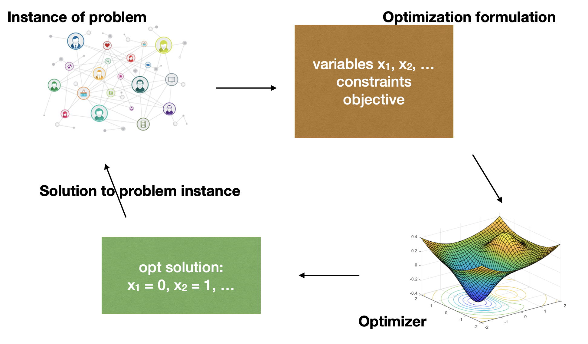
As discussed above, for the optimization formulation to be equivalent to the original problem, we must be able to convert any solution output by the optimizer to one of the original instance (while maintaining the cost).

More examples

In the examples above, it was almost "immediate" that the optimization formulation "exactly captures" the combinatorial problem we started out with (i.e., solutions to the original problem correspond exactly to the solutions to the optimization formulation). The next example illustrates that this step can sometimes be tricky.

Minimum spanning tree (MST). Recall the MST problem we discussed earlier in the course: we are given a weighted undirected graph $(V, E$) with non-negative weights $\{w_e\}_{e \in E}$ on the edges, and the goal is to pick the subset $S$ of the edges such that (a) all the vertices are connected, i.e., using only the edges $S$, there is a path from every vertex to every other vertex, (b) the total weight of the edges chosen is minimized.

At a high level the problem seems easy to phrase as optimization. We need to pick a subset of the edges, so suppose we have binary variables $x_e$, one for each edge $e$. The "intended" solution is to set $x_e=1$ if edge $e$ is picked and $0$ otherwise.

The objective is also easy: it is simply to minimize $\sum_{e \in E} w_e x_e$.

The tricky part is enforcing the constraint that using only the edges of $S$, there is a path from every vertex to every other vertex.

Idea 1: the first idea is to place conditions that "ensure" that the edges chosen form a tree. These can be: ones such as

• $(n-1)$ edges are chosen in total: $\sum_{e \in E} x_e = n-1$.
• Let $f_1, f_2, \dots, f_r \in E$ be the edges of any cycle in $G$. Then $x_{f_1} + x_{f_2} + \dots + x_{f_r} \le r-1$.
• $x_e \in \{0,1\}$

These conditions suffice to force the chosen set of edges to form a spanning tree (because the only way to select $n-1$ edges without having a cycle is to have a spanning tree -- this is a simple exercise if it's not clear).

Number of constraints. In the formulation above, the number of constraints is equal to the number of cycles in the graph, which is typically exponential in the number of vertices.

Idea 2: the above method is based on ensuring that we don't pick anything more than a tree. It did not explicitly enforce "connectivity between every pair" of vertices. It turns out that a nice way to enforce this is as follows:

• for every subset $T$ of the vertices that is not $\emptyset$ or $V$, let $\rho(T)$ denote the "boundary" of $T$, i.e., the set of edges that have one end-point in $T$ and another outside $T$. Now, for every $T$, we write the constraint: $\sum_{e \in \rho(T)} x_e \ge 1$.

Apart from this, we have the constraints $x_e \in \{0,1\}$, and the objective is as before.

We observe that if we had any set of values $\{x_e\}$ that satisfy the constraint above for all subsets $T$, then if we consider the graph $G'$ that only consists of the edges $e$ for which $x_e = 1$, $G'$ is connected. This can be argued as follows: suppose for the sake of contradiction that $G'$ is not connected. Then, consider some connected component of $G'$ and let its vertex set be $R$. By the definition of a connected component, $R$ has no edges to $V \setminus R$ in $G'$. But this means that $\{x_e\}$ doesn't satisfy the inequality $\sum_{e \in \rho(R)} x_e \ge 1$ -- a contradiction!

Efficient optimization

As we said before, if optimization formulations are to be useful for solving problems, the optimizer itself must be efficient. Indeed, as we said earlier, there are often many ways to express a problem as optimization, and the art is to choose one that can be solved easily using a solver.

It is therefore useful to know what kind of optimization problems can be solved efficiently in practice.

If we care about provably efficient procedures, perhaps the most important class is convex optimization, where the goal is to minimize a convex function over a convex set. For those of you interested in knowing more about these notions, please refer to the wikipedia page on convex optimization and Chapter 2 of these notes. There are also plenty of other notes online (and an extensive textbook by Boyd).

Linear programming

One special case of convex optimization is linear programming that we saw earlier. To recap, we have $n$ real valued variables $x_1, x_2, \dots, x_n$, and the objective is to maximize/minimize a linear function of these variables (i.e., a function of the form $c_1 x_1 + \dots + c_n x_n$, where $c_i$ are some (known) constants. Additionally, we have $m$ constraints that are also linear, i.e., the $i$'th constraint is $a_{i1} x_1 + a_{i2} x_2 + \dots + a_{in} x_n \le b_i$, where $a_{ij}$ and $b_i$ are again known constants. (This is succinctly written as $a_i^T x \le b_i$, as we view $a_i$ and $x$ as vectors.)

Linear programs have a nice geometry. Every constraint divides the entire space $\mathbb{R}^n$ into two "halves" (one side being feasible and another being infeasible). Thus, the feasible region for one constraint (say $a_i^T x \le b_i$) is often referred to as a half-space. The feasible set for the linear program is thus the intersection of $m$ half-spaces (one per constraint). The feasible region is called a "polytope". It can be either a bounded or an unbounded set; it can even be empty in which case the problem is said to be infeasible.

It turns out that many interesting problems arising in planning and operations research can be phrased as linear programming, and thus LPs are one of the most fundamental objects in optimization.

For a gentle introduction to linear programming (via examples in low dimension like we saw in class, refer to the excellent notes by Luca Trevisan).

Another nice feature of LPs is that the optimization can be solved in polynomial time. Indeed, this was a big open question until 1979, when the Soviet mathematician Khachiyan came up with a procedure known as the "Ellipsoid algorithm" which runs in time polynomial in the "input size" of the linear programming instance (polynomial in the bit complexities of the numbers $a_{ij}, b_i$ and $n, m$). Even though this was a theoretical breakthrough, in practice, a simpler "local search" procedure known as the "simplex algorithm" (which basically moves from one "vertex" of the polytope to a neighboring one in a systematic manner) works quite well in practice. More recently, a set of techniques collectively known as "interior point methods" have emerged as powerful alternatives to the simplex algorithm both in theory and in practice.

In what follows, we will treat the solution of LP as an efficient black-box, and see how this can help in solving combinatorial problems.

Combinatorial problems and "relaxations"

In the examples we saw earlier, we expressed problems such as matching, set cover and MST as optimization, but the variables involved were binary ones. In fact, in all of these examples, the constraints involved as well as the objective function were all linear (as we defined above), but the variables are binary, not real valued.

Such problems are called integer linear programs, or ILPs. While many heuristics exist for solving ILPs reasonably quickly, the problem is NP-hard, so we do not expect to have a general algorithm that scales well with the problem size.

Given that we care about algorithms with provable guarantees on the running time, does this mean that the optimization approach is useless?

The answer is no, because as we will see, we can often "relax" the binary constraints on the variables and still achieve meaningful insights into the problem. In what follows let us focus on a simple case of the set cover problem, namely the "vertex cover" question we saw earlier in the course.

Vertex cover. To recap, here we are given an undirected graph $G = (V, E)$, and the goal is to pick a subset $S$ of the vertices of the minimum possible size, such that for every edge $ij$, at least one of $i, j$ is in $S$. (This is a special case of Set Cover, if we view the vertices and edges as two sides of a bipartite graph.)

The optimization formulation for this problem (which is an ILP, as we saw before) is:

variables: $x_u$, $u \in V$.

objective: minimize $\sum_{u \in V} x_u$ subject to the constraints:

1. $x_u \in \{0,1\}$.
2. For all edges $ij$, $x_i + x_j \ge 1$

Now, the most natural way to convert this into a linear program is to replace the non-linear constraint (which is $x_u \in \{0,1\}$) with something linear, such as the constraint $0 \le x_u \le 1$ (to be clear, these are two linear constraints).

Thus the LP relaxation of the formulation above is:

minimize $\sum_{u \in V} x_u$ subject to:

1. $0 \le x_u \le 1$
2. for all edges $ij$, $x_i + x_j \ge 1$.

Comparing the objective values. The first thing to note is that both the original formulation (which we will call the ILP) and the relaxation are minimization problems. Further, every feasible solution to the ILP is also a feasible solution to the relaxation. In other words, the relaxation is a minimization over a "larger set" of solutions, and thus the optimum objective value of the relaxation is less than or equal to the optimum objective value of the ILP.

The natural question is if the optimum objective value of the relaxation is strictly smaller than that of the ILP. The answer is that it depends on the graph. For instance, consider the vertex cover problem when the graph is simply a triangle. Here, the minimum vertex cover has size $2$, and the ILP has optimum objective value equal to 2. But note that the solution $x_u = 1/2$ for all three vertices is feasible for the relaxation (it satisfies $0 \le x_u \le 1$, and also $x_i + x_j \ge 1$ for all edges). This solution has objective value equal to $3/2 = 1.5$.

Thus in this case, the opt objective value of the relaxation is strictly smaller than that of the ILP.

Such a gap between the objective value of the ILP and that of the relaxation is called the integrality gap of the formulation. One of the central themes in approximation algorithms is to come up with ILP formulations for different problems that have a (provably) small integrality gap. This way, even though the LP solution can be fractional (and thus may not be useful to recover a solution to the original problem), we have a decent estimate of the optimum objective value.

Rounding fractional solutions

Given the gap above, one may ask if for the vertex cover problem, there are instances in which the optimum objective value for the relaxation is way smaller than that of the ILP (say a factor 100 smaller).

We show now that the "gap" is always bounded by factor of 2. Further, we do this in a "constructive" way: given any feasible solution to the relaxation (which potentially has fractional values), we construct feasible solution to the ILP (i.e., a binary solution), with the guarantee that the objective value is not much larger. This process in general is known as rounding LP solutions.

Formally, suppose we have a feasible "fractional" solution $\{x_u\}$ for the LP relaxation above. We will construct a solution $\{y_u\}$ for the ILP (i.e. the original formulation), such that the objective values, namely $\sum_u x_u$ and $\sum_u y_u$ are not too far apart.

Rounding for vertex cover: let us consider the most "natural" rounding procedure: if $x_u \ge 1/2$, we set the corresponding $y_u$ to be 1, and if $x_u < 1/2$, we set $y_u = 0$. We do this for every $u \in V$.

Interestingly, in this case, the $\{y_u\}$ produced is in fact a feasible solution to the ILP! To check this, we only have to show that for every edge $ij$, $y_i + y_j \ge 1$. Why is this true? Observe that we started with a feasible (fractional) solution $\{x_u\}$ for the LP and rounded it to obtain $\{y_u\}$. Thus we know that $x_i + x_j \ge 1$. Now this means that at least one of $x_i, x_j$ should have been $\ge 1/2$, and by our rounding procedure, the corresponding $y$ value is $1$. Thus $y_i + y_j \ge 1$ for every edge!

Now, how can we compare $\sum_u y_u$ with $\sum_u x_u$? A simple upper bound can be obtained as follows: for every $u$, our rounding procedure implies that $y_u \le 2 x_u$. This is because if $x_u < 1/2$, then $y_u = 0$ so the above is trivially true. Otherwise, we have $x_u \ge 1/2$ and $y_u =1$, implying that $y_u \le 2x_u$.

Thus, summing over all $u$, we have $\sum_u y_u \le 2 \sum_u x_u$. This means that the feasible binary solution that we constructed (i.e., $\{y_u\}$) has objective value that is at most $2$ times that of the LP relaxation.

An approximation algorithm for Vertex cover

We will now see why the above implies a factor 2 approximation algorithm for the vertex cover problem. I.e., an algorithm that is guaranteed to output a solution whose objective value is at most two-times the optimum objective value. (Recall that we saw in one of our HWs that a "lazy" greedy algorithm also achieves this.)

The algorithm works as follows: given an instance $(V, E)$ of vertex cover (VC),

• first write down the ILP (i.e. our optimization formulation with binary variables); as we saw, there's a correspondence between solutions to this and those of the VC instance.
• now write down the LP relaxation. This is a linear program, so we solve it in polynomial time (say using Khachiyan's algorithm). Let $\{ x_u\}$ be the optimum solution.
• perform rounding to obtain $\{y_u\}$ -- a feasible solution to the ILP, and then output the corresponding solution to the VC problem.

Now, how do we compare the solution output by the algorithm to the optimum one? Suppose the objective value of the optimum solution to the VC instance $(V, E)$ is $OPT$. Then the ILP we write down in the first step also has optimum value $OPT$ (as it captures the VC instance exactly). Next, as we argued earlier (in the section introducing relaxations), the optimum objective value of the LP relaxation --suppose it is denoted $OPT_{LP}$-- is smaller than or equal to $OPT$. Thus, for the optimum solution $x$, we have $\sum_u x_u \le OPT$. Now, using the argument we made for rounding, we have that $\sum_u y_u \le 2 \cdot OPT$, which is what we claimed.

Just as an example, in the case where the instance is a triangle, starting with the solution $x_u = 1/2$ for all vertices, the rounding algorithm ends up picking all three vertices of the triangle (thus achieving an objective value of $3$, which is sub-optimal, but not by much).

Relax and round. The above process is an example of a more general framework, known as relax-and-round. It is a powerful framework for designing approximation algorithms for combinatorial optimization problems. The first step is to write down an ILP formulation involving (typically) binary variables. The next step is to "relax" the constraints to obtain a Linear program, which can be solved in polynomial time using an LP solver. This results in a potentially "fractional" solution. The last step is to "round" the fractional solution to a binary one, obtaining a feasible solution to the ILP. This is then used to obtain a solution to the original problem.

Set cover and randomized rounding